Setting up the analysis (step 5)

1. We are now ready to set up some parameters before starting the quantitative analysis. The main idea is to guide in the right direction the final solution for what concearning the parameters that are easy to be checked by viewing the spectrum.
2. From the 'Refinement' menu, click on the 'Compute spectrum' option. This will allow the program to compute a spectrum with the actual values of the parameters.
3. Now, go to the "Datasets" tabPanel in the main MAUD window and select our dataset. Click on the 'Edit' button and go to the "Datafiles' tabPanel. Select the file you loaded before and click on the 'View' button. A new window will appear showing the experimental datapoint (blue) and the fitting (black).
4. Click on the 'Change parameter' option in the 'Update' menu and a new window called "Live parameters" will show up (see the next figure).
   
   
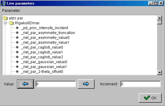
   Live parameters frame
   
   Now, you will be able to modify real time the fitting increasing or decreasing the value of the parameters. Arrange the plot and the "Live parameters" windows in order to see both at the same time. In the "Our dataset" object, select the "riet_par_background_pol0" field. Input an increment of 10 in the "Increment" field and  increment the intensity to 40 by using the right arrow.
5. Now scroll up to the beginning of the "Live parameters" frame. In the "RigakuIIIDmax" object select the "pd_proc_intensity_incident" field (incident intensity). Input an increment of 10 in the "Increment" field and  increment the intensity value by using the right arrow. The following figure shows you what you should have obtained after this first step.
   
   
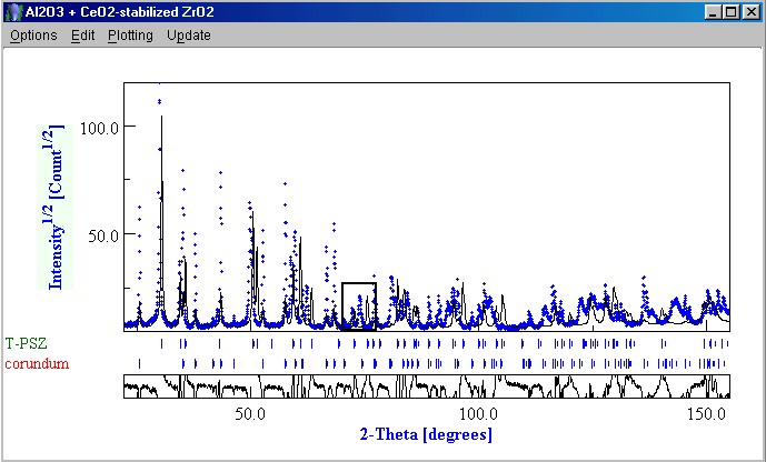
   Plot frame
   
   As you notice, the T-PSZ peaks are shifted due to wrong cell parameters for this phase. We can zoom in a small region of the spectrum to control more efficientely what is going on. Drag a rectangular window using the mouse to zoom in around the peaks between 70 and 80 degrees, as shown in the previous figure.
6. Once you have zoomed in, go back to the "Live parameters" window and scroll down to the T-PSZ object. Select the "_cell_length_c" cell parameter, input an increment of 0.005 in the "Increment" field and start shifting the 400 peak by clicking on the right arrow (we are increasing the parameter's value). After a good overlapping of the experimental and calculated peaks, select the "_cell_length_a" cell parameter of the T-PSZ. Repeat the same procedure until you get a good overlapping for the 220 reflection. The two following figures show the fitted profile before and after the procedures.
   
   
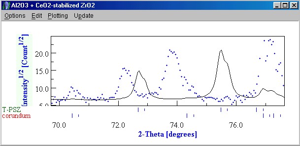
   Zoomed-in plot window before changes
   
   
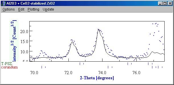
   Zoomed-in plot window after changes
   
   Close the "Live parameters" window and zoom out  the plot window by double-clicking on it. Your plot should be similar to the one in the next figure.
   
   
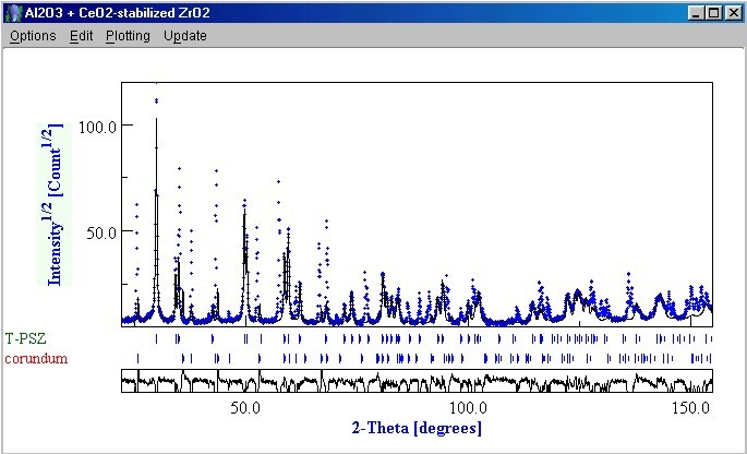
   Good fitting after changing the T-PSZ cell parameters
   
   Close the plot window and then the "Datasets" tabPanel by clicking on 'OK' button. Now, you are ready for the analysis.